M.A. Cross

Everyone has their guilty pleasures, myself included. One of them, among many others that shall forever remain secret, is the 2011 drama Margin Call. It's a really solid movie to be fair, but I find myself thinking about it a disproportionate amount. I really like how perfect the dialogue is — everyone strings together their thoughts in a smooth, coherent performance that makes me wonder if I'm even speaking the same language as these dudes. That one dialogue between Jeremy Irons and Zachary Quinto specifically occupies an embarrassingly large part of my mind.

Anyway, all of this is to say that I've had that Wall Street slickness on my mind for some time, so when the need arose to practice some NumPy (for work), I thought I'd role play as our friend Peter Sullivan in the Risk Analysis and Management office and do some market modeling.

The Plan

I would like to point out, before we begin, that the goal here was to get comfortable with NumPy and vectorization, NOT to come up with a viable trading strategy. I need to stress this now so when you see my model get rinsed by the S&P 500 you feel a little less bad for me.

With that said, the plan is straightforward. For our target stock/fund: take a long-term moving average and a short-term moving average. When the short-term average is greater than our long-term average, we hold. When the short-term average dips below the long-term average, we sell. Nice and simple.

The Recipe

For my model, I downloaded 5 years worth of SPY into a csv, then trimmed off everything but dates and closing prices.

The data set I used had dates in monotonic decreasing, so I had to flip those around.

    df = pd.read_csv('HistoricalData.csv')
    # Select date and Close/last columns and order them in ascending order 
    data = df[["Date", "Close/Last"]].to_numpy()[::-1]  
    if not valid_data(data):
        raise ValueError("Invalid data")

    dates = data[:, 0]  # Extract dates
    prices =  data[:, 1].astype(float)  # Convert prices to float
    returns = np.diff(prices) / prices[:-1]  # Calculate returns

To calculate returns, we do (closing price today − closing price yesterday) / (closing price yesterday). This is called a simple return, and it's going to serve as our control in this experiment. It would be equivalent to if I bought a share of SPY at the start of our dataset and held it all the way to the end.

    returns = np.diff(prices) / prices[:-1] 

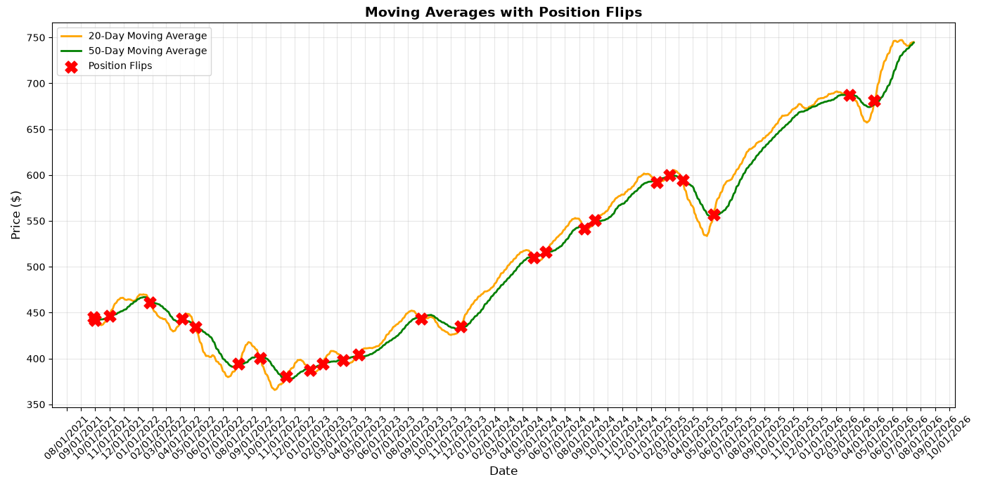
In order to get our moving averages, we need to slide a window through our prices. The size of our window determines the number of days that factor into our average. More days = a longer average. I'm sure there's a lot that goes into picking good window sizes, but I arbitrarily picked 20 days and 50 days for our short and long moving averages respectively.

    # Calculate 20-day moving average
    short_ma = sliding_window_view(prices, window_shape=20).mean(axis=1)  
    # Calculate 50-day moving average
    long_ma = sliding_window_view(prices, window_shape=50).mean(axis=1)

Note the first n days for our window of size n go into calculating the first point in our average. Therefore, we need to crop off the first n - 1 days from any dataset we want to compare to our moving averages. In this case, we crop to match a window of 50 days.

    # Crop first 30 days off short_ma to align with long_ma
    short_ma = short_ma[30:]
    dates_cropped = dates[49:]  # Start from day 50 (index 49)
    prices_cropped = prices[49:]

At this point we have everything we need to derive our positions. There's a bit of nuance here in that all of our math is done on the closing price of our stock. IRL this means that the market is closed by the time we are able to derive each point in our model, meaning it wouldn't make sense to trade on the same day that the short+long averages are calculated. We therefore shift all of our positions once to the right.

    # Identify long signals (1 for long, 0 for short)
    long_signals = (short_ma > long_ma).astype(int)  
    # update position off previous day's signal
    position = np.concatenate([[0], long_signals[:-1]]) 
    # Calculate portfolio returns based on position 
    portfolio_returns = position * returns  

The Fruits of Our Labor

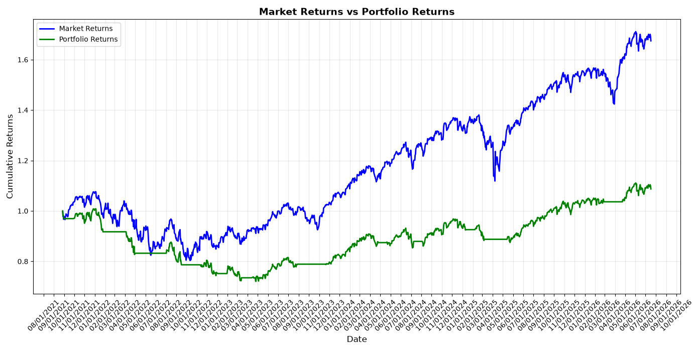
To be fair, what did you expect. If a 21-year old could beat the S&P 500 in an afternoon with 10 lines of python code, I think we would all be in trouble. You can get the gist from eyeballing the graph, but here's some more stats on just how badly we performed.

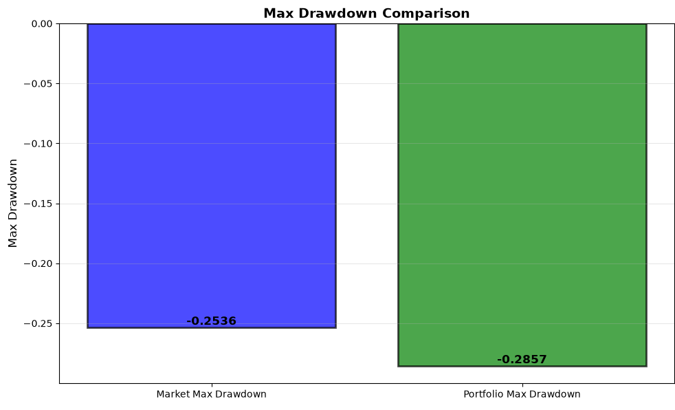
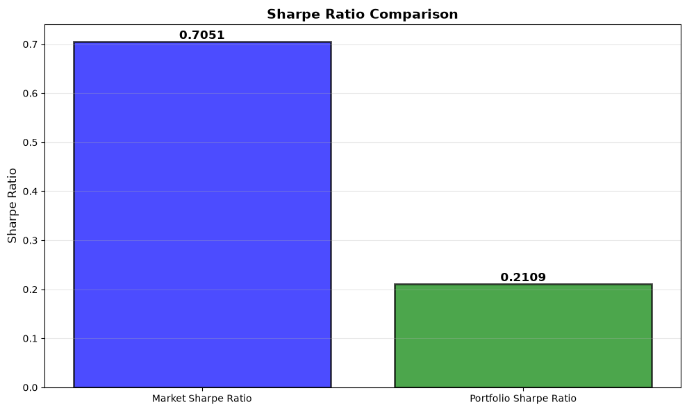
What I did find interesting was the lack of look-ahead bias. Remember earlier when I said I shifted our positions forward a day since we should be trading on the previous days findings? If I didn't do that my model would have something called "look-ahead bias", which should inflate our returns a decent amount. I plotted our model with that bias, and we are still underperforming the S&P, which I thought was strange. Here's the plot with the biased returns:

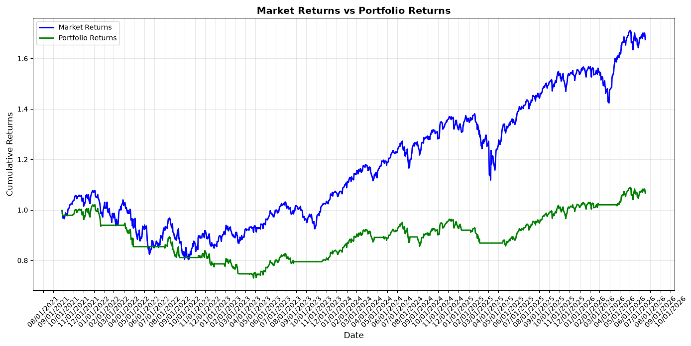
It looks almost identical to our original. After plotting the actual points where our position flips, I think it's due to the fact that the S&P has been growing so steadily over the last 5 years. We only ever flipped our position 25 times, and look-ahead bias only gives an advantage when a position is flipped, so I suppose that makes sense. Had I picked a more volatile dataset the results could have been more interesting.

Anyhow, I came in hoping to get more comfortable with NumPy and that's exactly what I did so I can't be too mad. Maybe one day I'll be dealing with models that end up beating the S&P, in which case I will NOT be publishing a guide on how that works. For now, I think I'll keep my savings comfortably in an index fund. Adieu!